When a new ham eventually wants to get on HF, the antenna is usually the biggest source of difficulty. For a lot of people, it is often not practical to make and use an HF antenna that is self resonant due to the large size. For example, if we wanted to make a half-wave dipole for the 20m band, it would have to be 10m across, which is massive! So here enters electrically short transmitting antennas; antennas which are able to transmit on a given frequency while being less than 1/4 of the wavelength, albeit with some notable tradeoffs which we will see later.
Desired Antenna Specifications
So, some form of compromise antenna, something electrically shortned, is in order. To make this not entirely hopeless, I decided that I would build something to operate primarily on the 10m band, with the ability of tuning to lower bands but with reduced efficiency. Below I list additional specifications that were desirable.
- Portable: Given that I live in a small apartment most of the year, I want the antenna to be portable so I can take it somewhere outdoors to perform contacts.
- Cheap to build: As per ham tradition, I wanted to make it using only junk and hardware store parts.
- Low loss: This constraint is a consequence of constraint 1.: Since we’re portable, we’re also QRP, and since we are QRP we don’t have much wattage to spare, hence we want to minimize losses where possible. Based on these requirements, I decided to go with a magnetic loop antenna design. At first, I was hoping to use a design that someone had already made and that met these requirements, but I thought it would be more fun to read up on the theory and design my own.
Theory
I’ll start by going over the math I did to get my antenna build specifications but feel free to skip this section if math scares you.
Magnetic loop antennas employ inductive coupling and tuned resonance to achieve relatively good transmitting performance on wavelengths much larger than the antenna’s physical size. But, as always in physics, there is no free lunch. The catch is that the antenna must be tuned to a given frequency with a variable capacitor and, once tuned, often has a very narrow bandwidth. Additionally, the radiation resistance of a small loop is often very small, making it very important to reduce the AC resistance in the antenna in order to achieve good efficiency. Minimizing the AC resistance, however, has the unfortunate consequence of narrowing your bandwidth, so the trick is to strike a good balance.
We first calculate the loop’s self inductance
$$ L=\mu_0\left(\log\left(\frac{8R}{r}\right)-2+\frac{r^2}{R^2}\left(-\frac{1}{8}\log\left(\frac{8R}{r}\right)+\frac{5}{24}\right)\right) $$where $\mu_0$ is the permeability of free space, $R$ is the radius of the loop and $r$ is the radius of the copper pipe. This is a highly accurate approximation for the inductance taken from the widely used text by F.W. Grover. For a 6ft circumference loop with 1/2” copper pipe we get a self inductance value of $\sim 1.35 \mu\text{H}$.
Now the antenna can be viewed as a tuned RLC circuit. Knowing the inductance, we can easily determine the required capacitance to tune to a given frequency $f$.
$$ C=\frac{1}{4\pi^2Lf^2} $$For a 6ft loop at the middle of the 10m band, we get a required capacitance of about $22 \text{ pF}$.
Estimated Performance
Although the actual efficiency will be much lower due to additional AC resistance from connection points to the capacitor and potential loose connectors, it is still helpful to visualize at what rate the efficiency decays. To do so, we need to determine the radiation and AC resistance of the antenna. The radiation resistance is given by
$$ R_r = 320\pi^4\left(\frac{na}{\lambda^2}\right)^2 $$where $a$ is, interestingly, the area of the loop, $n$ the number of turns and $\lambda$ the wavelength of operation. We then compute the AC resistance
$$ R_{AC} = \frac{1}{\sigma\pi d \delta(f)}l $$where $\sigma$ is the conductivity of copper ($58 \text{ MS/m}$), $d$ is the diameter of our copper pipe, $l$ is the length of our loop and $\delta(f)$ is the skin depth as a function of frequency $f$, given by
$$ \delta(f) = \sqrt{\frac{\rho}{\pi f\mu_0 \mu_r}} $$with $\rho$ being the inverse of conductivity ($1/\sigma$), $\mu_0$ being the permeability of free space, and $\mu_r$ being the relative permeability of the conductor (0.999 for copper).
Plotting these two equations as a function of frequency, we can see that although the AC resistance depends on the frequency due to the skin effect, it doesn’t vary anywhere near as much as the radiation resistance does.
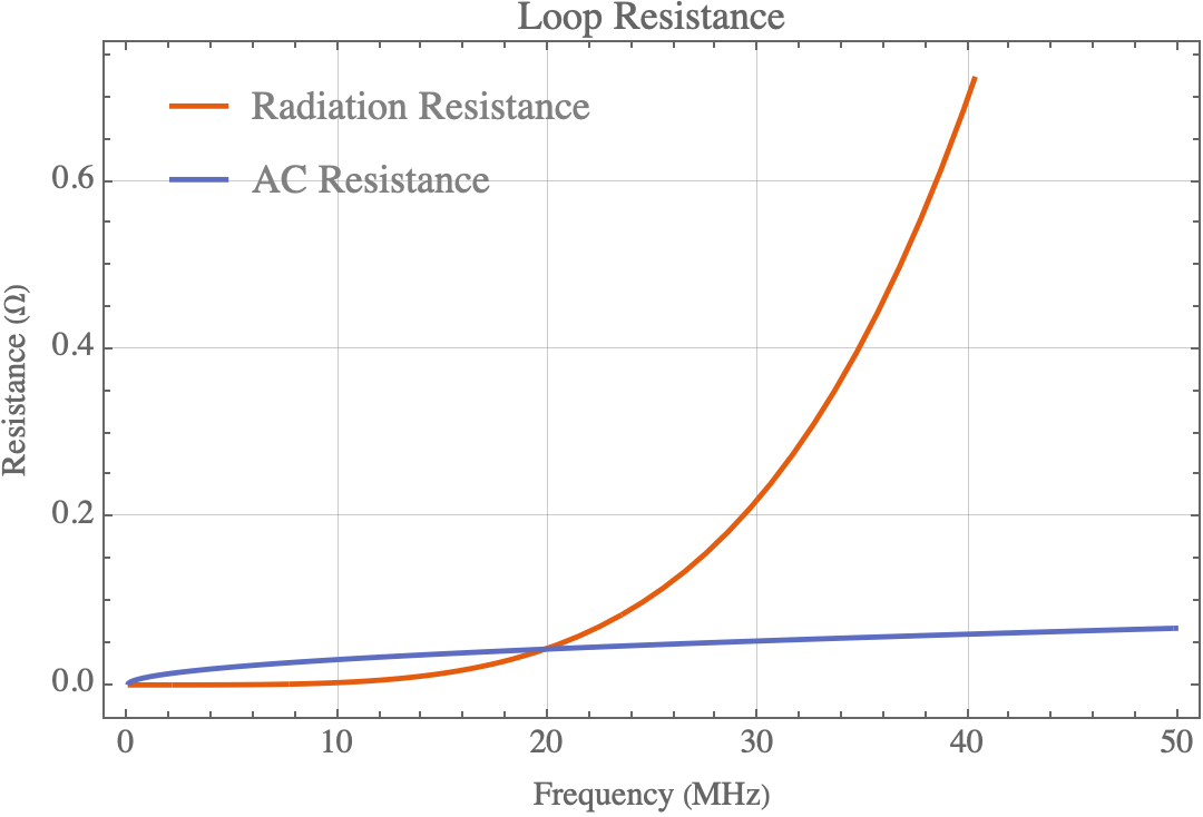 Something cool to notice is how the frequency where the radiation resistance equals the AC Resistance corresponds to the same frequency at which our efficiency is 50%.
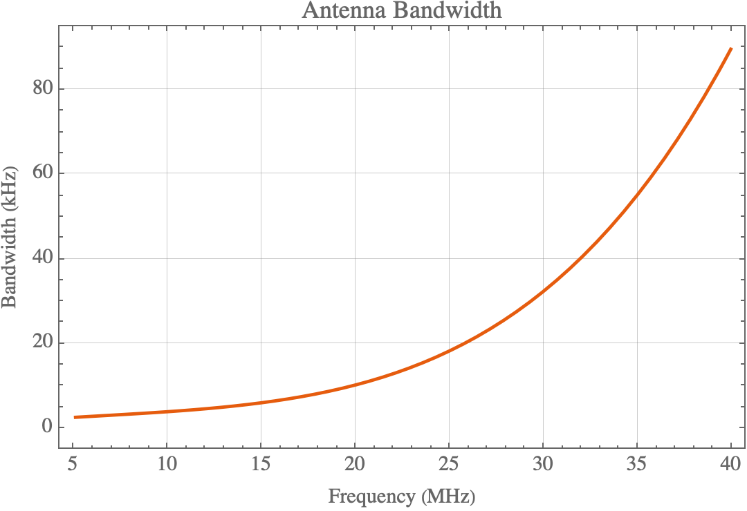
Since the antenna is basically an RLC circuit we can compute the quality factor and thus the bandwidth. First, we get the capacitor’s reactance $X$:
$$ X = \frac{1}{2\pi(f C)} $$where $f$ is the operating frequency and $C$ is the capacitance. Then the quality factor is given by
$$ Q = \frac{X}{R_r + R_{AC}} $$where $R_r$ and $R_{AC}$ are the radiation and AC resistances respectively. The bandwidth is then just
$$ \Delta f = f/Q $$
Importantly, Q is a function of three things that are also functions of frequency, so we have to plug them all in to each other, a messy exercise in algebra that I will omit here. Anyway, we can see that the bandwidth of the antenna is perfectly usable at every frequency we would be using this antenna on.
 Finally, we can look into the antenna’s estimated efficiency, which is a function of radiation resistance and AC resistance:
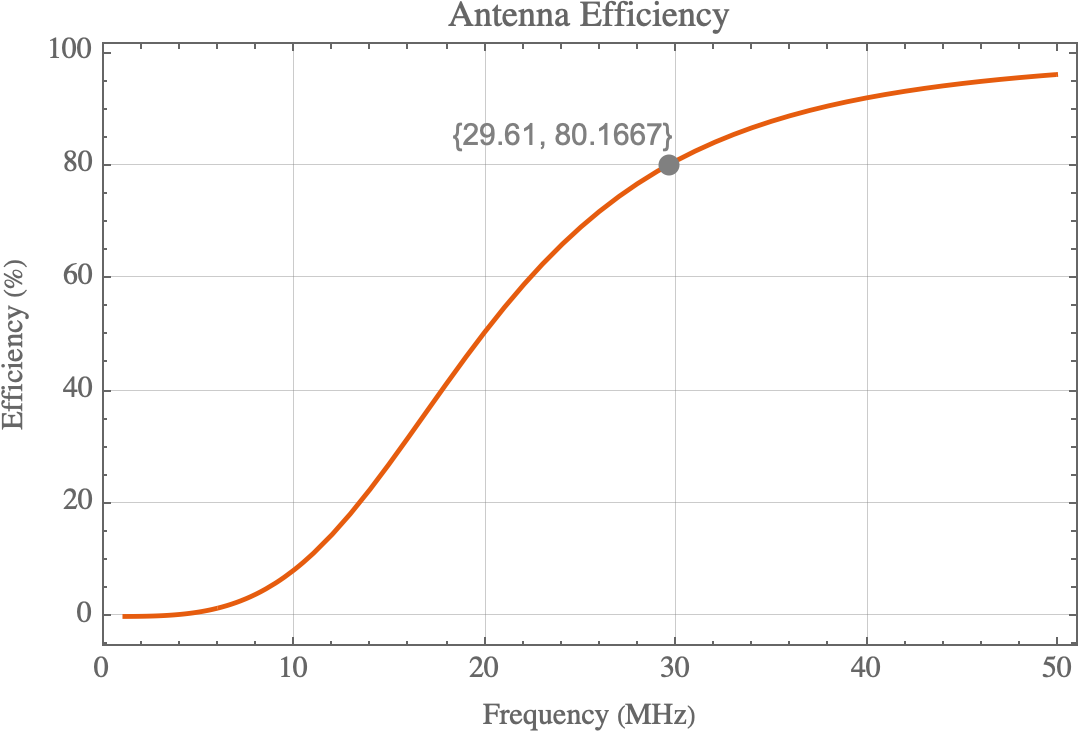 We can see that the antenna’s efficiency decreases dramatically as we lower the frequency. This curve can be flattened out by either decreasing the AC resistance or increasing the radiation resistance. To decrease the AC resistance, we can either increase the pipe diameter or minimize losses in other parts of the antenna. Increasing the radiation resistance has a more significant effect and is oftentimes easier since we can do so by simply building a loop with a larger circumference.
Construction
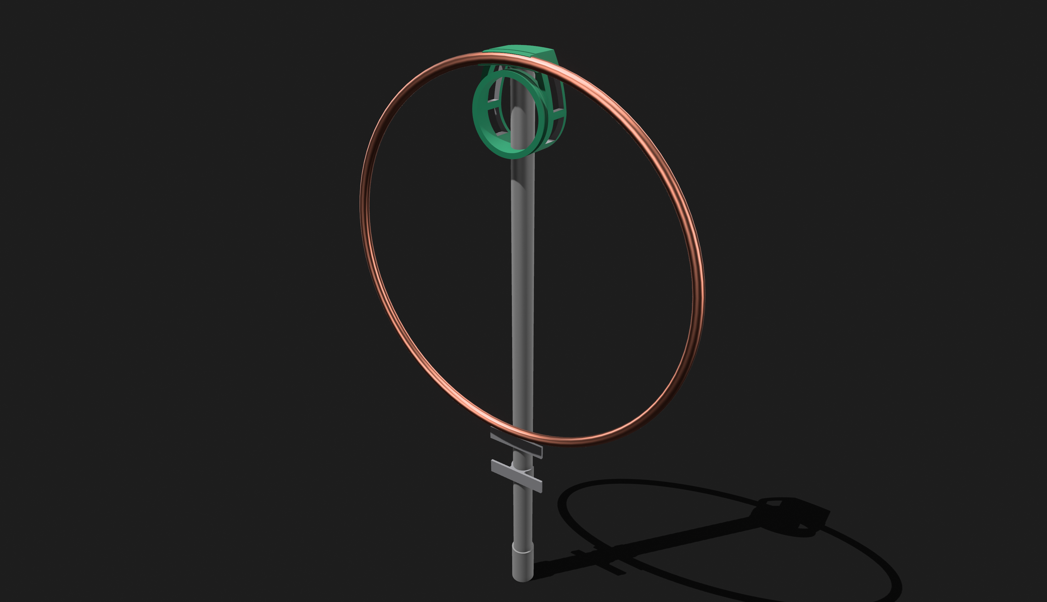
I’ve seen a lot of different ways people build magnetic loops online. Square, hexagonal, and octagonal loops seem to be pretty popular when using solid copper pipe, but they all require soldering every joint and, as I found out when I went to the hardware store, copper elbows are expensive, especially if you have to buy eight of them. So I decided to find a way to bend copper pipe into a circle instead. As a bonus, a circle is the most performant shape for a loop antenna as it maximizes the enclosed area for a given length of pipe.
Main Loop
Contrary to what I was told by the hardware store employee, it actually is possible to bend 1/2” copper pipe. To bend it into a circle I’ll refer you to the tutorial I followed. Building the rig to get this pipe bent into a circle wasn’t easy, but if you have more experience in wood working than I do you shouldn’t have much trouble.
Warning: you should make sure to anneal the copper pipe before trying to bend it. I forgot to do this at first, and in the following pictures you will see where I kinked the pipe. Annealing requires heating the copper to a certain temperature and letting it cool slowly.
After going back and forth between different loop circumferences I decided on 6ft as it gave a quite portable size without sacrificing too much performance. We gain some portability while still getting an estimated 80% efficiency on the 10m band. We’ll use 1/2” Type M copper pipe . Note that there is more than one type of 1/2” copper pipe sold in stores. From what I could tell they all have the same outer diameter but with varying wall thicknesses. The thicker walled pipe might offer a small gain in efficiency, but I was unsure about its ability to be bent, so I went with thin walled (Type M) copper pipe. As a bonus the thinner walled pipe is quite a bit cheaper.
Inner Loop
The magnetic loop of course requires a smaller loop that is about 1/5 the circumference of the main loop. This smaller loop is what will actually be driven by our transceiver. For this I made two different designs, one using 6 gauge automotive battery wire and the other with copper refrigeration tubing. We want something that is hefty here as the thicker the wire the lower the AC resistance. To keep the inner loop close to the main loop I designed a 3D printed bracket that snaps onto the main loop and holds the inner loop in a circular shape. This bracket also holds the main and inner loop to a segment of PVC pipe.
Capacitor
From the calculated self-inductance of the main loop, we can determine that we need about 22.60 pF of capacitance for the antenna to tune to 28.85 MHz. I’m cheap, so I decided to make my own variable capacitor. Ideally, due to the high voltages involved, the design shouldn’t have any wiper contacts (metal sliding on metal). These can be problematic due to arcing and can also become a significant source of electrical loss. In a butterfly capacitor, the two halves that are connected to the antenna are fixed, whereas the rotor is not electrically connected to the rest of the circuit. By turning the rotor, we change how much overlap there is between plates and therefore the capcitance. The downside is that, in this configuration, the capacitor plates are connected in series, which gives us less capacitance than if we had connected them in parallel, but as we’ve seen this entire antenna is a story of tradeoffs.
Following another instructables tutorial and using an old piece of aluminum plate found in my dad’s shed, we cut a total of 27 plates: 18 stators and 9 rotors. This aluminum plate is a little over 1mm thick. The plates are then drilled with a hole big enough for 8-32 threaded rod, and the plates are stacked on rods with 8-32 nuts and washers spacing them and holding them in place. The end result is a basic homemade butterfly capacitor which gives a maximum capacitance of about 53 pF .
 Based off of the dimensions of the PVC pipe that I wanted to mount the antenna to, I designed mounting clips that could be zip tied to the capacitor’s end brackets. A tuning knob was also printed to insulate the capacitor from the user.
Empirical Results
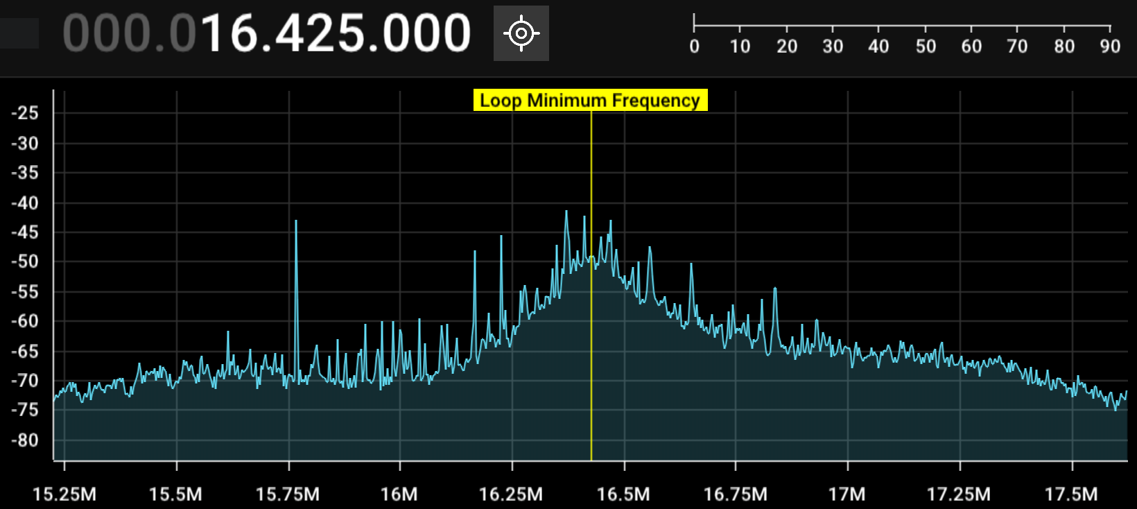
As it turns out, the bandwidth of the antenna is actually far wider and shallower than my calculations would suggest. This was to be expected as the idealized calculations do not take into effect the resistance from the terminal connections to the capacitor. Using an RTL-SDR, you can actually see the frequency to which the antenna is tuned, and even at its lowest possible tuning frequency, the peak is not very sharp.
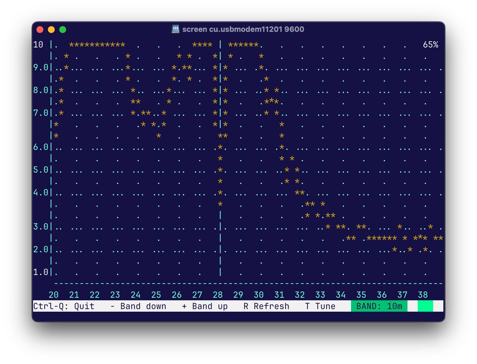
As for the SWR, when tuned properly I was able to get it as low as 1.2, but its peak is very narrow, as you can see in the picture below.
 As for transmitting performance, I was able get multiple QSOs on FT8 with operators as far as Poland from my kitchen on 5W. On PSKReporter I was even heard as far as Antartica, again still in my kitchen and with only 5W.
Conclusion
Although the efficiency is probably not great and the portability questionable, this antenna has surpased my expectations of what can be done with compact electrically short antennas. It was also a good starting point and was a great learning experience. Of course, there are many improvements that I already know can be made to make this antenna even better. Most notably, squishing the inner loop into an oval shape so as to maximize the amount of length that is in proximity to the main loop can apparently greatly increase efficiency.
Parts List (Not exhaustive)
- (1) 6ft 1/2" Copper Pipe ~$14
- (1) 2ft Automotive battery wire 4 gauge ~$11
- (2) Battery leads to connect capacitor to loop
- (1) Silver solder
- (1) PETG 3D printing filament
- (1) Aluminum Sheet Metal ~$15
- (8) 8-32 Hex nuts
- (1) 8-32 1ft threaded rod
- (1) BNC Connector
Required tools
- Jigsaw
- 3D Printer
- Saw for cutting sheet aluminum
References
https://vk8rhradioprojects.com/magnetic-loop-antennas/ ARRL Antenna Book 21st Edition Vol 2. Griffith’s E&M Calculations and plots made with the help of Wolfram Mathematica